Chapter 6.1.2 Simulation Case Studies

Randomization case studies

Randomization is a statistical technique suitable for evaluating whether a difference in sample proportions is due to chance. In this section, we explore the situation where we focus on a single proportion, and we introduce a new simulation method.

dvds

How rational and consistent is the behavior of the typical American college student? In this section, we’ll explore whether college student consumers always consider an obvious fact:
money not spent now can be spent later.
In particular, we are interested in whether reminding students about this well-known fact about money causes them to be a little thriftier. A skeptic might think that such a reminder would have no impact. We can summarize these two perspectives using the null and alternative hypothesis framework.
H0: Null hypothesis. Reminding students that they can save money for later purchases will not have any impact on students’ spending decisions.
Ha: Alternative hypothesis. Reminding students that they can save money for later purchases will reduce the chance they will continue with a purchase.
In this section, we’ll explore an experiment conducted by researchers that investigates this very question for students at a university in the southwestern United States.

Exploring the data set before the analysis

One-hundred and fifty students were recruited for the study, and each was given the following statement:
Imagine that you have been saving some extra money on the side to make some purchases, and on your most recent visit to the video store you come across a special sale on a new video. This video is one with your favorite actor or actress, and your favorite type of movie (such as a comedy, drama, thriller, etc.). This particular video that you are considering is one you have been thinking about buying for a long time. It is available for a special sale price of $14.99.
What would you do in this situation? Please circle one of the options below.

Half of the 150 students were randomized into a control group and were given the following two options:
(A) Buy this entertaining video.
(B) Not buy this entertaining video.

The remaining 75 students were placed in the treatment group, and they saw a slightly modified option (B):
(A) Buy this entertaining video.
(B) Not buy this entertaining video. Keep the $14.99 for other purchases.

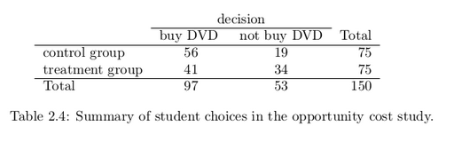
Would the extra statement reminding students of an obvious fact impact the purchasing decision? Table 2.4 summarizes the study results.

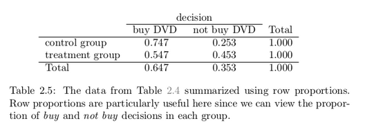
It might be a little easier to review the results using row proportions, specifically considering the proportion of participants in each group who said they would buy or not buy the DVD. These summaries are given in Table 2.5.

We will define as success in this study as a student who chooses not to buy the DVD.

Success is often defined in a study as the outcome of interest, and a “success” may or may not actually be a positive outcome. For example, researchers working on a study on HIV prevalence might define a
“success” in the statistical sense as a patient who is HIV+. A more complete discussion of the term success will be given in Chapter 3.

Then, the value of interest is the change in DVD purchase rates that results by reminding students that not spending money now means they can spend the money later. We can construct a point estimate for this difference as

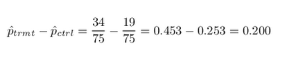
The proportion of students who chose not to buy the DVD was 20% higher in the treatment group than the control group. However, is this result statistically significant? In other words, is a 20% difference between the two groups so prominent that it is unlikely to have occurred from chance alone?

Results from chance alone

The primary goal in this data analysis is to understand what sort of differences we might see if the null hypothesis were true, i.e. the treatment had no effect on students. For this, we’ll use the same procedure we applied in Section 2.1: randomization.
Let’s think about the data in the context of the hypotheses. If the null hypothesis (H0) was true and the treatment had no impact on student decisions, then the observed difference between the two groups of 20% could be attributed entirely to chance. If, on the other hand, the alternative hypothesis (H A ) is true, then the difference indicates that reminding students about saving for later purchases actually impacts their buying decisions.
Just like with the gender discrimination study, we can perform a statistical analysis. Using the same randomization technique from the last section, let’s see what happens when we simulate the experiment under the scenario where there is no effect from the treatment.
While we would in reality do this simulation on a computer, it might be useful to think about how we would go about carrying out the simulation without a computer. We start with 150 index cards and label each card to indicate the distribution of our response variable: decision. That is, 53 cards will be labeled “not buy DVD” to represent the 53 students who opted not to buy, and 97 will be labeled “buy DVD” for the other 97 students. Then we shuffle these cards throughly and divide them into two stacks of size 75, representing the simulated treatment and control groups. Any observed difference between the proportions of “not buy DVD” cards (what we earlier defined as success) can be attributed entirely to chance.

If we are randomly assigning the cards into the simulated treatment
and control groups, how many “not buy DVD” cards would we expect to end up with in each simulated group? What would be the expected difference between the proportions of “not buy DVD” cards in each group?

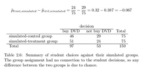
Answer: Since the simulated groups are of equal size, we would expect 53/2 = 26.5, i.e. 26 or 27, “not buy DVD” cards in each simulated group, yielding a simulated point estimate of 0%. However, due to random fluctuations, we might actually observe a number a little above or below 26 and 27.

The results of a randomization from chance alone is shown in Table 2.6. From this table, we can compute a difference that occurred from chance alone:

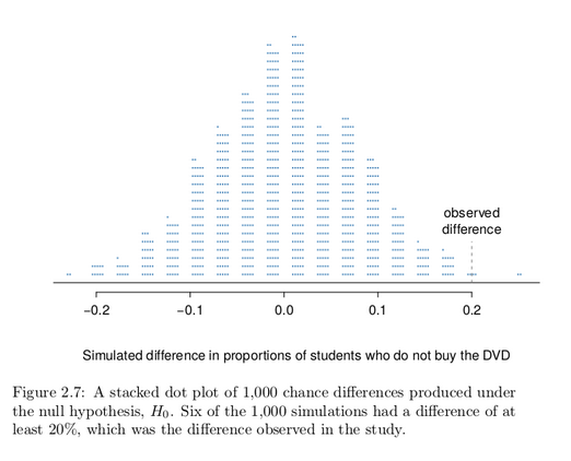
Just one simulation will not be enough to get a sense of what sorts of differences would happen from chance alone. We’ll simulate another set of simulated groups and compute the new difference: 0.013. And again: 0.067. And again: -0.173. We’ll do this 1,000 times. The results are summarized in a dot plot in Figure 2.7, where each point represents
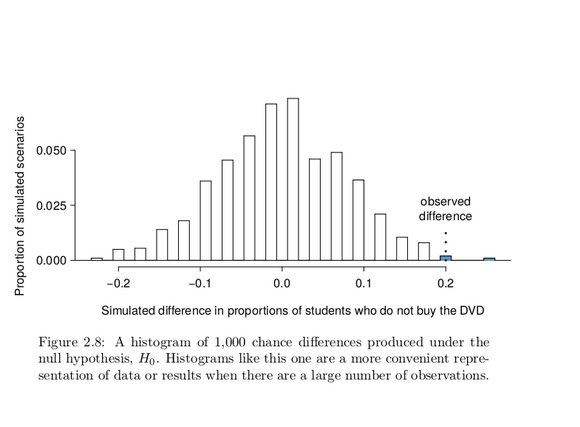
a simulation. Since there are so many points, it is more convenient to summarize the results in a histogram such as the one in Figure 2.8, where the height of each histogram bar represents the fraction of observations in that group.
If there was no treatment effect, then we’d only observe a difference of at least +20% about 0.6% of the time, or about 1-in-150 times. That is really rare! Instead, we will conclude the data provide strong evidence there is a treatment effect: reminding students before a purchase that they could instead spend the money later on something else lowers
the chance that they will continue with the purchase. Notice that we are able to make a causal statement for this study since the study is an experiment.

Gender Discrimination

We consider a study investigating gender discrimination in the 1970s, which is set in the context of personnel decisions within a bank. 2 The research question we hope to answer is, “Are females discriminated against in promotion decisions made by male managers?”

Variability within data

The participants in this study were 48 male bank supervisors attending a management institute at the University of North Carolina in 1972. They were asked to assume the role of the personnel director of a bank and were given a personnel file to judge whether the person should be promoted to a branch manager position. The files given to the participants were identical, except that half of them indicated the candidate was male and the other half indicated the candidate was female. These files were randomly assigned to the subjects.

Is this an observational study or an experiment? How does
the type of study impact what can be inferred from the results?

The study is an experiment, as subjects were randomly assigned a male file or a female file. Since this is an experiment, the results can be used to evaluate a causal relationship between gender of a candidate
and the promotion decision.

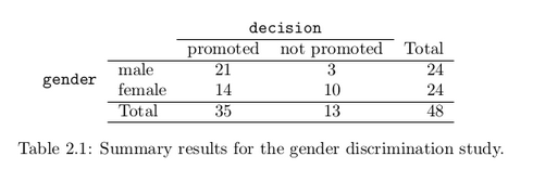
For each supervisor we recorded the gender associated with the assigned file and the promotion decision. Using the results of the study summarized in Table 2.1, we would like to evaluate if females are unfairly discriminated against in promotion decisions. In this study, a smaller proportion of females are promoted than males (0.583 versus 0.875), but
it is unclear whether the difference provides convincing evidence that females are unfairly discriminated against.

Statisticians are sometimes called upon to evaluate the strength of
evidence. When looking at the rates of promotion for males and females in this study, why might we be tempted to immediately conclude that females are being discriminated against?
The large difference in promotion rates (58.3% for females versus 87.5% for males) suggest there might be discrimination against women in promotion decisions. However, we cannot yet be sure if the observed difference represents discrimination or is just from random chance. Generally there is a little bit of fluctuation in sample data, and we wouldn’t expect the sample proportions to be exactly equal, even if the truth was that the promotion decisions were independent of gender.
Example 2.4 is a reminder that the observed outcomes in the sample may not perfectly reflect the true relationships between variables in the underlying population. Table 2.1 shows there were 7 fewer promotions in the female group than in the male group, a difference in promotion rates of 29.2% (21/24− 14/24=0.292). This observed difference is what we call a point estimate of the true effect. The point estimate of the difference is large, but the sample size for the study is small, making it unclear if this observed difference represents discrimination or whether it is simply due to chance. We label these two competing claims, H0 and Ha :

H0 : Null hypothesis. The variables gender and decision are independent. They have no relationship, and the observed difference between the proportion of males and females who were promoted, 29.2%, was due to chance.
Ha : Alternative hypothesis. The variables gender and decision are not independent. The difference in promotion rates of 29.2% was not due to chance, and equally qualified females are less likely to be promoted than males.

These hypotheses are part of what is called a hypothesis test. A hypothesis test is a statistical technique used to evaluate competing claims using data. Oftentimes, the null hypothesis takes a stance of no difference or no effect. If the null hypothesis and the data notably disagree, then we will reject the null hypothesis in favor of the alternative hypothesis.

What would it mean if the null hypothesis, which says the variables gender and decision are unrelated, is true? It would mean each banker would decide whether to promote the candidate without regard to the gender indicated on the file. That is, the difference in the promotion percentages would be due to the way the files were randomly divided to the bankers, and the randomization just happened to give rise to a relatively large difference of 29.2%.
Consider the alternative hypothesis: bankers were influenced by which gender was listed on the personnel file. If this was true, and especially if this influence was substantial, we would expect to see some difference in the promotion rates of male and female candidates. If this gender bias was against females, we would expect a smaller fraction of promotion recommendations for female personnel files relative to the male files. We will choose between these two competing claims by assessing if the data conflict so much with H0 that the null hypothesis cannot be deemed reasonable. If this is the case, and the data support Ha , then we will reject the notion of independence and conclude that these data provide strong evidence of discrimination.

Simulating the study

Table 2.1 shows that 35 bank supervisors recommended promotion and 13 did not. Now, suppose the bankers’ decisions were independent of gender. Then, if we conducted the experiment again with a different random assignment of files, differences in promotion rates would be based only on random fluctuation. We can actually perform this randomization, which simulates what would have happened if the bankers’ decisions had been independent of gender but we had distributed the files differently.

The test procedure we employ in this section is formally called a permutation test.

In this simulation, we thoroughly shuffle 48 personnel files, 24 labeled male and 24 labeled female, and deal these files into two stacks. We will deal 35 files into the first stack, which will represent the 35 supervisors who recommended promotion. The second stack will have 13 files, and it will represent the 13 supervisors who recommended against promotion. Then, as we did with the original data, we tabulate the results and determine the fraction of male and female who were promoted.
Since the randomization of files in this simulation is independent of the promotion decisions, any difference in the two fractions is entirely due to chance. Table 2.2 show the results of such a simulation.

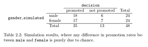
What is the difference in promotion rates between the two simulated groups in Table 2.2? How does this compare to the observed difference
29.2% from the actual study?

18/24 − 17/24 = 0.042 or about 4.2% in favor of the men. This difference due to chance is much smaller than the difference observed in the actual groups.

Checking for independence

We computed one possible difference under the null hypothesis in Guided Practice 2.5, which represents one difference due to chance. While in this first simulation, we physically dealt out files, it is much more efficient to perform this simulation using a computer.
Repeating the simulation on a computer, we get another difference due to chance: -0.042. And another: 0.208. And so on until we repeat the simulation enough times that we have a good idea of what represents the distribution of differences from chance alone.

Figure 2.3 shows a plot of the differences found from 100 simulations, where each dot represents a simulated difference between the proportions of male and female files recommended for promotion.

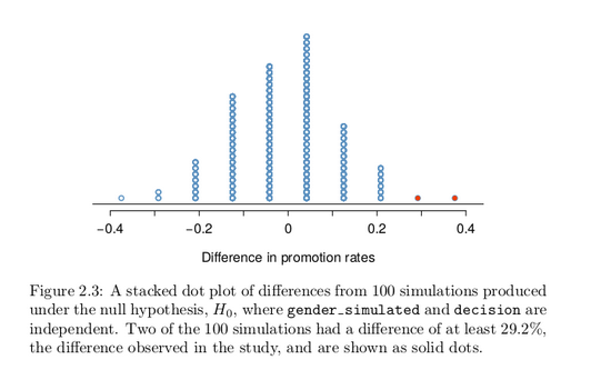
Note that the distribution of these simulated differences is centered around 0. Because we simulated differences in a way that made no distinction between men and women, this makes sense: we should expect differences from chance alone to fall around zero with some random fluctuation for each simulation.

How often would you observe a difference of at least 29.2% (0.292)
according to Figure 2.3? Often, sometimes, rarely, or never?

It appears that a difference of at least 29.2% due to chance alone would only happen about 2% of the time according to Figure 2.3. Such a low probability indicates that observing such a large difference from chance is rare.

The difference of 29.2% is a rare event if there really is no impact from listing gender in the candidates’ files, which provides us with two possible interpretations of the study results:
H 0 : Null hypothesis. Gender has no effect on promotion decision, and we observed a difference that is so large that it would only happen rarely.
H A : Alternative hypothesis. Gender has an effect on promotion decision, and what we observed was actually due to equally qualified women being discriminated against in promotion decisions, which explains the large difference of 29.2%.

When we conduct formal studies, we reject a skeptical position if the data strongly conflict with that position.

This reasoning does not generally extend to anecdotal observations. Each of us observes incredibly rare events every day, events we could not possibly hope to predict. However, in the non-rigorous setting of
anecdotal evidence, almost anything may appear to be a rare event, so the idea of looking for rare events in day-to-day activities is treacherous. For example, we might look at the lottery: there was only a 1 in 176 million chance that the Mega Millions numbers for the largest jackpot in history (March 30, 2012) would be (2, 4, 23, 38, 46) with a Mega ball of (23), but nonetheless those numbers came up! However, no matter
what numbers had turned up, they would have had the same incredibly rare odds. That is, any set of numbers we could have observed would ultimately be incredibly rare. This type of situation is typical of our
daily lives: each possible event in itself seems incredibly rare, but if we consider every alternative, those outcomes are also incredibly rare. We should be cautious not to misinterpret such anecdotal evidence.

In our analysis, we determined that there was only a ≈2% probability of obtaining a sample where ≥29.2% more males than females get promoted by chance alone, so we conclude the data provide strong evidence of gender discrimination against women by the supervisors. In this case, we reject the null hypothesis in favor of the alternative.

Statistical inference is the practice of making decisions and conclusions from data in the context of uncertainty. Errors do occur, just like rare events, and the data set at hand might lead us to the wrong conclusion. While a given data set may not always lead us to a correct conclusion, statistical inference gives us tools to control and evaluate how often these errors occur. Before getting into the nuances of hypothesis testing, let’s work through another case study.

Simulation case studies

Medical consultant

People providing an organ for donation sometimes seek the help of a special medical consultant. These consultants assist the patient in all aspects of the surgery, with the goal of reducing the possibility of complications during the medical procedure and recovery.
Patients might choose a consultant based in part on the historical complication rate of the consultant’s clients.

One consultant tried to attract patients by noting the average complication rate for liver donor surgeries in the US is about 10%, but her clients have had only 3 complications in the 62 liver donor surgeries she has facilitated. She claims this is strong evidence that her work meaningfully contributes to reducing complications (and therefore she should be hired!).

We will let p represent the true complication rate for liver donors
working with this consultant. Estimate p using the data, and label this value p̂.

The sample proportion for the complication rate is 3 complications divided by the 62 surgeries the consultant has worked on: p̂ = 3/62 = 0.048.

Q & A

Is it possible to assess the consultant’s claim using the data?

No. The claim is that there is a causal connection, but the data are observational. For example, maybe patients who can afford a medical consultant can afford better medical care, which can also lead to a lower complication rate.
While it is not possible to assess the causal claim, it is still possible to test for an association using these data. For this question we ask, could the low complication rate of p̂ = 0.048 be due to chance?

We’re going to conduct a hypothesis test for this setting. Should
the test be one-sided or two-sided?

The setting has been framed in the context of the consultant being helpful, but what if the consultant actually performed worse than the average? Would we care? More than ever! Since we care about a finding in either direction, we should run a two-sided test.

Write out hypotheses in both plain and statistical language to test for the association between the consultant’s work and the true complication rate, p, for this consultant’s clients.

H0 : There is no association between the consultant’s contributions and the clients’ complication rate. That is, the complication rate for the consultant’s clients is equal to the US average of 10%. In statistical
language, p = 0.10.

Ha: Patients who work with the consultant have a complication rate different than 10%, i.e. p != 0.10.

Parameter for a hypothesis test:

A parameter for a hypothesis test is the “true” value of interest. We typically estimate the parameter using a point estimate from a sample of data.
For example, we estimate the probability p of a complication for a client of the medical consultant by examining the past complications rates of her clients: p̂ = 3/62 = 0.048 is used to estimate p

Null value of a hypothesis test:

The null value is the reference value for the parameter in H0, and it is sometimes represented with the parameter’s label with a subscript 0, e.g. p0 (just like H0).

In the medical consultant case study, the parameter is p and the null value is p 0 = 0.10. We will use the p-value to quantify the possibility of a sample proportion (p̂) this far from the null value. The p-value is computed based on the null distribution, which is the distribution of the test statistic if the null hypothesis were true. Just like we did using randomization for a difference in proportions, here we can simulate 62 new patients to see what result might happen if the complication rate was 0.10.
Each client can be simulated using a deck of cards. Take one red card, nine black cards, and mix them up. If the cards are well-shuffled, drawing the top card is one way of simulating the chance a patient has a complication if the true rate is 0.10: if the card is red, we say the patient had a complication, and if it is black then we say they did not have a complication. If we repeat this process 62 times and compute the proportion of simulated patients with complications, p̂ sim , then this simulated proportion is exactly a draw from the null distribution.

In a simulation of 62 patients, about how many would we expect to have had a complication?

About 10% of the patients (6.2 on average) in the simulation will have a complication, though we will see a little variation from one simulation to the next.

We conducted such a simulation. There were 5 simulated cases with a complication and 57 simulated cases without a complication: p̂sim = 5/62 = 0.081.
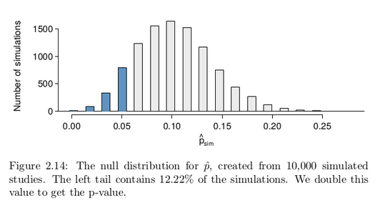
One simulation isn’t enough to get a sense of the null distribution, so we repeated the simulation 10,000 times using a computer. Figure 2.14 shows the null distribution from these 10,000 simulations. The simulated proportions that are less than or equal to p̂ = 0.048 are shaded. There were 1222 simulated sample proportions with p̂sim ≤ 0.048, which represents a fraction 0.1222 of our simulations:

left tail =Number of observed simulations with p̂sim ≤ 0.048 / 10000
=1222 / 10000
= 0.1222

However, this is not our p-value! Remember that we are conducting a two-sided test, so we should double the one-tail area to get the p-value:
p-value = 2 × left tail = 2 × 0.1222 = 0.2444.

This doubling approach is preferred even when the distribution isn’t symmetric, as in this case.

Because the p-value is 0.2444, which is larger than the significance level 0.05, we do not reject the null hypothesis. Explain what this means
in the context of the problem using plain language.

The data do not provide strong evidence that the consultant’s work is associated with a lower or higher rate of surgery complications than the general rate of 10%.

Does the conclusion in Guided Practice 2.23 imply there is no real
association between the surgical consultant’s work and the risk of complications? Explain.
No. It might be that the consultant’s work is associated with a lower or higher risk of complications. However, the data did not provide enough information to reject the null hypothesis.

Tappers and listeners

Here’s a game you can try with your friends or family: pick a simple, well-known song, tap that tune on your desk, and see if the other person can guess the song. In this simple game, you are the tapper, and the other person is the listener.
A Stanford University graduate student named Elizabeth Newton conducted an experiment using the tapper-listener game. In her study, she recruited 120 tappers and 120 listeners into the study. About 50% of the tappers expected that the listener would be able to guess the song. Newton wondered, is 50% a reasonable expectation?
Newton’s research question can be framed into two hypotheses:

H0: The tappers are correct, and generally 50% of the time listeners are able to guess the tune. p = 0.50
Ha: The tappers are incorrect, and either more than or less than 50% of listeners will be able to guess the tune. p != 0.50

In Newton’s study, only 3 out of 120 listeners (p̂ = 0.025) were able to guess the tune! From the perspective of the null hypothesis, we might wonder, how likely is it that we would get this result from chance alone? That is, what’s the chance we would happen to see such a small fraction if H0 were true and the true correct-guess rate is 0.50?

We will again use a simulation. To simulate 120 games under the null hypothesis where p = 0.50, we could flip a coin 120 times. Each time the coin came up heads, this could represent the listener guessing correctly, and tails would represent the listener guessing incorrectly. For example, we can simulate 5 tapper-listener pairs by flipping a coin 5 times:

H H T H T
Correct Correct Wrong Correct Wrong

After flipping the coin 120 times, we got 56 heads for p̂sim = 0.467.

As we did with the randomization technique, seeing what would happen with one simulation isn’t enough. In order to evaluate whether our originally observed proportion of 0.025 is unusual or not, we should generate more simulations. Here we’ve repeated this simulation ten times:
0.558 0.517 0.467 0.458 0.525 0.425 0.458 0.492 0.550 0.483

As before, we’ll run a total of 10,000 simulations using a computer. Figure 2.15 shows the results of these simulations. Even in these 10,000 simulations, we don’t see any results close to 0.025.

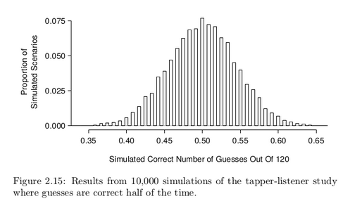
What is the p-value for the hypothesis test?

The p-value is the chance of seeing the data summary or something more in favor of the alternative hypothesis. Since we didn’t observe anything even close to just 3 correct, the p-value will be small, around
1-in-10,000 or smaller.

Do the data provide statistically significant evidence against the null hypothesis? State an appropriate conclusion in the context of the research question.

The p-value is less than 0.05, so we reject the null hypothesis. There is statistically significant evidence, and the data provide strong evidence that the chance a listener will guess the correct tune is less than 50%.