Chapter 1.2.4.2 Estimating Continuous Distributions

In this section, we show how to estimate the pdf of a continuous rv via simulation. As opposed to the discrete case, we will not get an explicit formula for the pdf, but we will rather get a graph of it.

Example Estimate the pdf of $2Z$ when $Z$ is a standard normal random variable

Our strategy is to take a random sample of size 10,000 and use the R function geom_density inside of ggplot2 to estimate the pdf. As before, we build our sample of size 10,000 up as follows:

A single value sampled from standard normal rv:

z <- rnorm(1)

We multiply it by 2 to get a single value sampled from $2Z$ .

2 * z

## [1] -0.05017198

Now create 10,000 values of $2Z$ :

zData <- 2 * rnorm(10000)

We then use ggplot to estimate and plot the pdf of the data, after converting to a data frame:

ggplot(data.frame(zData), aes(x = zData)) + geom_density()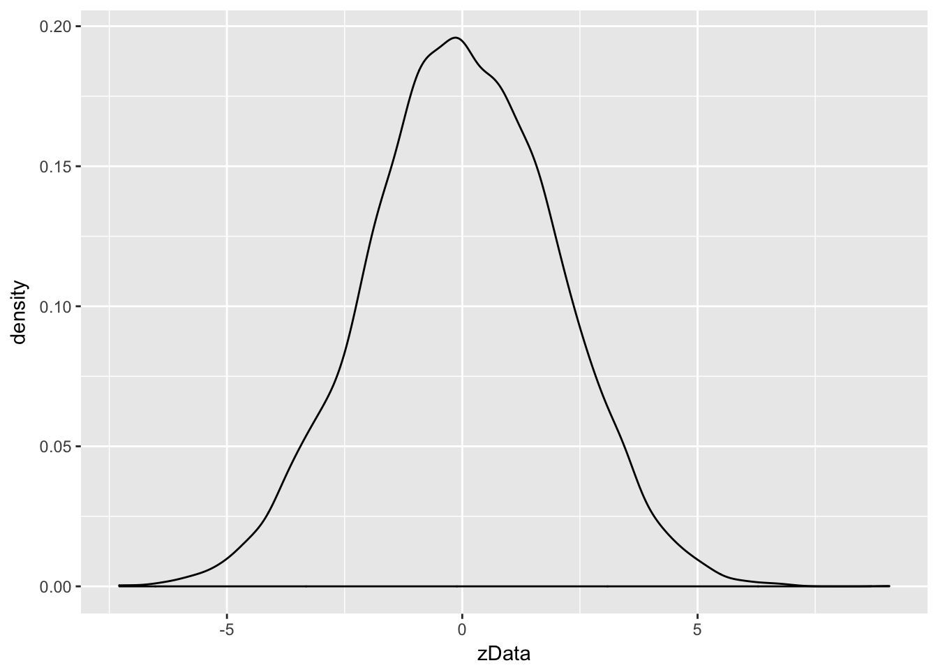

Notice that the most likely outcome of $2Z$ seems to be centered around 0, just as it is for $Z$ , but that the spread of the distribution of $2Z$ is twice as wide as the spread of $Z$ .

Example Estimate via simulation the pdf of $log(|Z|)$ when $Z$ is standard normal.

expData <- log(abs(rnorm(10000)))
ggplot(data.frame(expData), aes(x = expData)) + geom_density()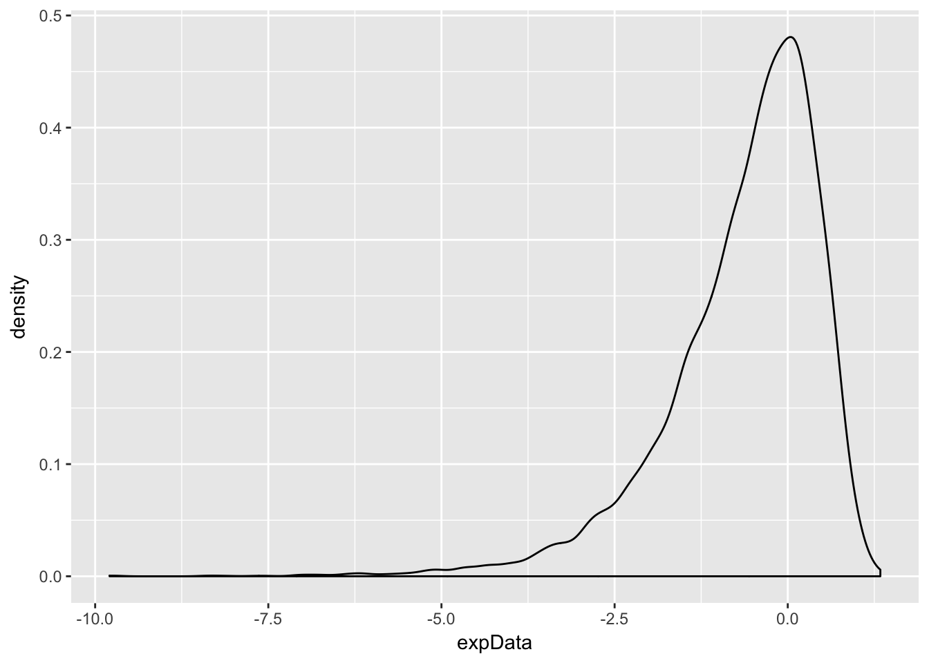

Both of the above worked pretty well, but there are issues when your pdf has discontinuities. Let’s see.

Example Estimate the pdf of $X$ when $X$ is uniform on the interval $[-1,1]$ .

unifData <- runif(10000,-1,1)
ggplot(data.frame(unifData), aes(x = unifData)) + geom_density()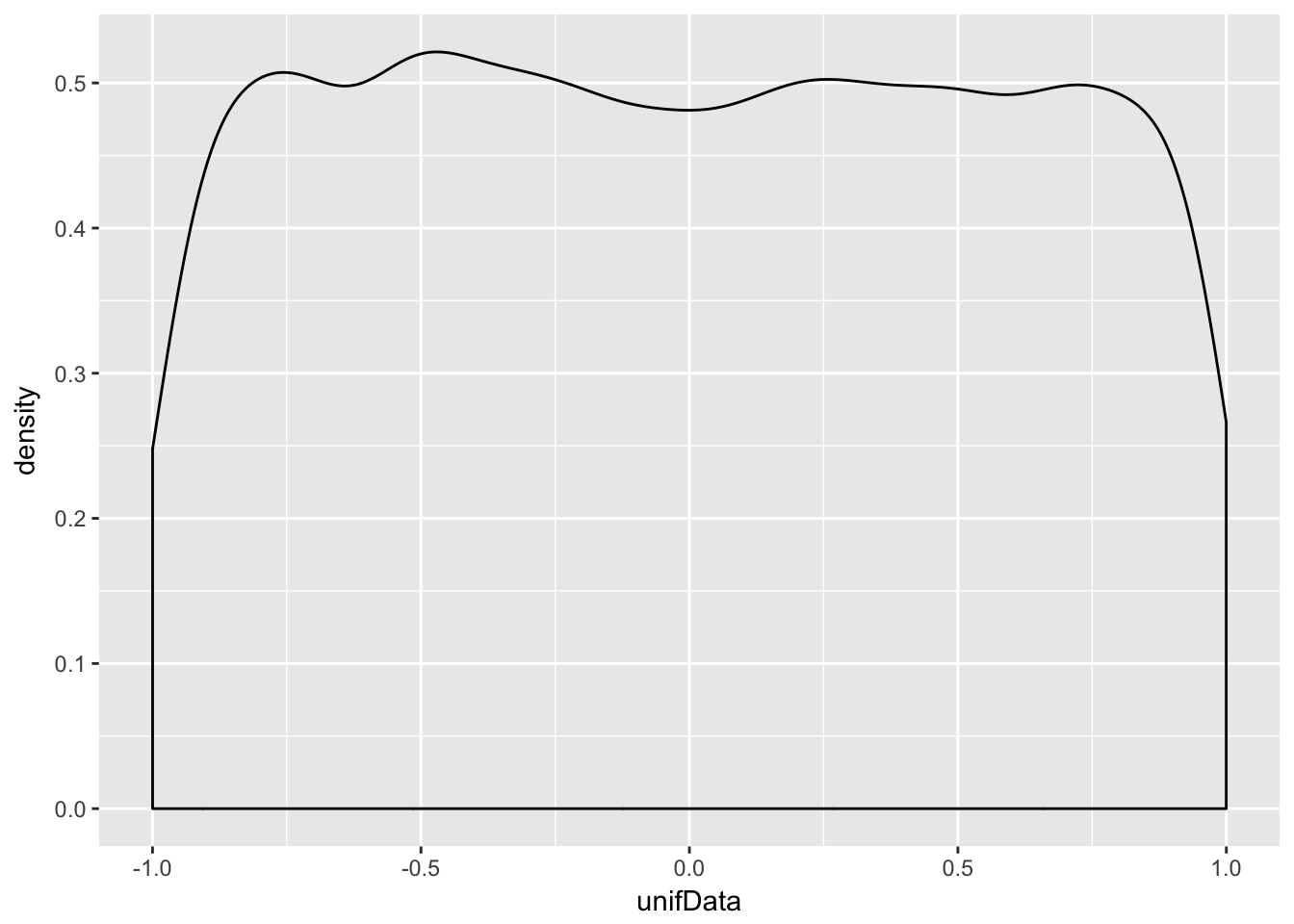

This distribution should be exactly 0.5 between -1 and 1, and zero everywhere else. The simulation is reasonable in the middle, but the discontinuities at the endpoints are not shown well. Increasing the number of data points helps, but does not fix the problem.

Example Estimate the pdf of $X2X^2$ when $XX$ is uniform on the interval $[-1,1][-1,1]$ .

X2data <- runif(10000,-1,1)^2
ggplot(data.frame(X2data), aes(x = X2data)) + geom_density()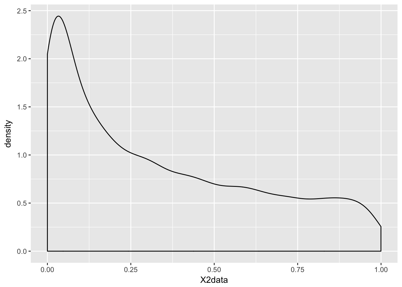

Example Estimate the pdf of $X+YX + Y$ when $XX$ and $YY$ are exponential random variables with rate 2.

X <- rexp(10000,2)
Y <- rexp(10000,2)
sumData <- X + Y
ggplot(data.frame(sumData), aes(x = sumData)) + geom_density()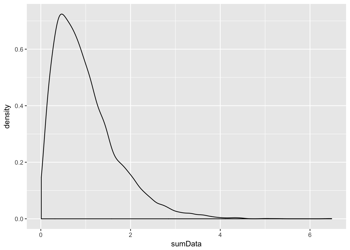

Example Estimate the density of $X1+X2+⋯+X20X_1 + X_2 + \cdots + X_{20}$ when all of the $XiX_i$ are exponential random variables with rate 2.

This one is trickier and the first one for which we need to use replicate to create the data. Let’s build up the experiment that we are replicating from the ground up.

Here’s the experiment of summing 20 exponential rvs with rate 2:

sum(rexp(20,2))

## [1] 10.74181

Now, we replicate it (10 times to test):

replicate(10, sum(rexp(20,2)))

##  [1] 11.046925 10.993640 11.597361 10.745458 10.653840 10.304673 11.596451
##  [8] 14.613796  6.608730  9.030899

Of course, we don’t want to just replicate it 10 times, we need about 10,000 data points to get a good density estimate.

sumExpData <- replicate(10000, sum(rexp(20,2)))
ggplot(data.frame(sumExpData), aes(x = sumExpData)) + geom_density()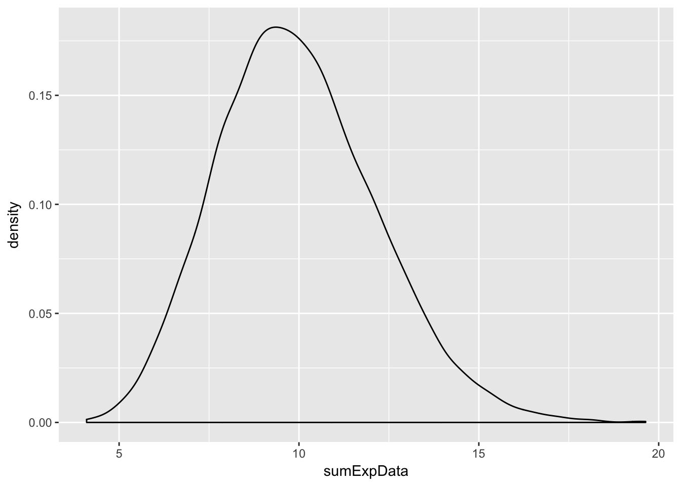

Note that this is starting to look like a normal random variable!!